Custom eBird Needs Lists

Ever wished the eBird website would take your state or county lists and tell you what you’re missing? What birds you need, ranked by how easily they might be found in a given state or county during a given week?  Well this past weekend I finally sat down and rigged some R code to do just that!

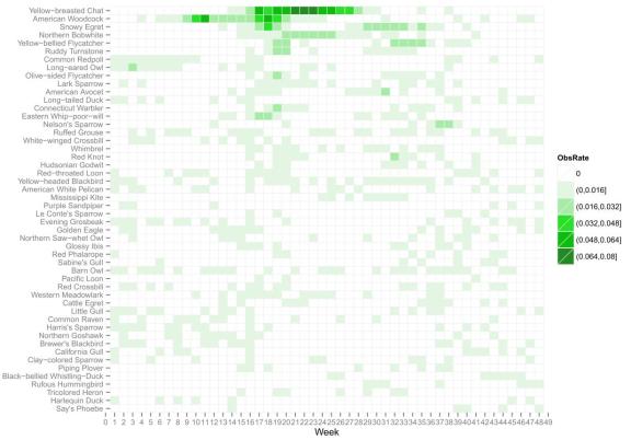
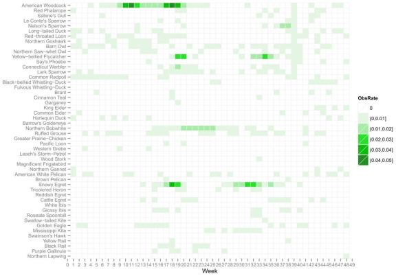
Here are my top 50 target birds according to the eBird data, ranked in the first/top figure by frequency of reports in eBird throughout the entire year, and ranked in the second/bottom figure by frequency of reports over the time period from last “week” (quarter month) through 2 “weeks” from now. If you were wondering, the last week in October is Week 39.

Top 50 Target Birds for Ohio (ranked by annual occurrence).

Top 50 Target Birds for Ohio (ranked by annual occurrence over week 38-41.

So how’d I make these? I’m glad you asked! A copy of the R script that does all the work can be found below, so without hitting all the details here is a sketch of the process.

First, I went ebird.org and downloaded my Ohio life list as a CSV file (renamed List.csv). Second, I went to the Bar Chart tool under the Explore Data portion of the website, pulled up the Ohio state list, and downloaded the histogram data (an MS Excel file). This file needed a little clean-up, as the header is full of empty rows and extra data, so these header rows were chopped so that the first row in the spreadsheet is the first row of data. That spreadsheet was then converted to a CSV file (BarChart.csv).

What the script then does is open up these files, chop the species names down to just the common name, cut out species group, hybrids, etc., the match up species names and see what’s left in the full Ohio list (my target birds!). The rest is just using the barchart info to reorder that list by how commonly those species are reported either in a given time span or cumulatively throughout the year.

## Generate a "hit list" based on a "life list" CSV download (unedited) from eBird
## and a comparable region barchart (edited to be just species rows, no titles).

## Birds I've seen
LIST = read.csv("List.csv");

## Barchart data
BARCHART = read.csv("BarChart.csv", header=F, colClasses=c("character",rep("numeric",12*4)));

## Take out rows of hybrids (hybrid), "spuhs" (sp.) and Combos (Sp1/Sp2)
BARCHART = BARCHART[grep("hybrid",BARCHART[,1],invert=TRUE),]
BARCHART = BARCHART[grep("sp\\.",BARCHART[,1],invert=TRUE),]
BARCHART = BARCHART[grep("[a-zA-Z]/[a-zA-Z]",BARCHART[,1],invert=TRUE),]

## Clean up the naming differences between LIST & BARCHART:
##    Barchart = Greater White-fronted Goose (<em class="sci">Anser albifrons</em>)
##    List     = Greater White-fronted Goose - Anser albifrons
## By chopping at " (" and " - ", respectively.
LIST[,2] = gsub(' \\- .+',"",LIST[,2]); 
BARCHART[,1] = gsub(' \\(.+',"",BARCHART[,1]); 

## Now compare species lists!
# BARCHART[!(BARCHART[,1] %in% LIST[,2]),1]
NeedsChart = BARCHART[!(BARCHART[,1] %in% LIST[,2]),]

## Get date info
month = as.numeric(format(Sys.time(), "%m")); # Get numeric month
week = ceiling(as.numeric(format(Sys.time(), "%d"))/31*4); # get approximate "week" 1,2,3 or 4

## Sort the whole thing by the current week, label columns
NeedsChart = NeedsChart[order(NeedsChart[,(month-1)*4+week+1], decreasing=T),]
names(NeedsChart) = c("Species",sapply(1:(12*4), function(x) paste("Week.",x,sep='')))
NeedsChart$Species = factor(NeedsChart$Species, levels=NeedsChart$Species); rownames(NeedsChart) = c();

## Or specify month and week here:
# month = 1; # 1,2,...,12
# week  = 1; # 1,2,3 or 4

## Or next week
# week = week+1;

## Or in the coming 3 weeks, plus hopes for stragglers from last week
week = -1:2 + week;

## Aggregate data
# First, rowSums is smart, but dumb.  Extend to handle single rows

HitList = data.frame(Species=NeedsChart[,1], 
                      Rate=as.matrix(rowSums(as.matrix(NeedsChart[,1+(month-1)*4+week])))   )
HitList = HitList[order(HitList$Rate,decreasing=T),]; rownames(HitList)=c();
## Cut species not observed in this timeframe?
HitList = HitList[HitList[,2]>0,]; 


## Plot part of NeedsChart
library(ggplot2) # for plotting tools
library(reshape2)# for melt() to reformat our data to use ggplot2

Nspecies=50 # How many species in the heat map?
Nbins   = 6 # How many colors/bins for the heat map?

# Stick with current weeks ranking (comment out), or go for annual rate (uncomment)?
NeedsChart = NeedsChart[order(rowSums(NeedsChart[,-1]),decreasing=T),]; rownames(HitList)=c();

# reformat the data for ggplot2's geom_tile() 
NC = melt(head(NeedsChart,Nspecies)); names(NC) = c("Species","Week","ObsRate");
NC$Week = as.numeric(gsub("Week\\.","",NC$Week)); 
NC$ObsRate = cut(NC$ObsRate, c(-1,seq(0,max(NC$ObsRate),length=Nbins))); # Bin data
levels(NC$ObsRate)[1] = "0"; # all positive, so (-1,0] == [0,0] == 0.

## Make a heat map using the ggplot2 geom_tile() aesthetic
base_size = 10 # font for lapels
my.palette = colorRampPalette(c("white", "#d0f0d0", "#00dd00", "forestgreen"))

g = ggplot(NC, aes(Week, Species)) + geom_tile(aes(fill=ObsRate), colour = "#f0f0f0") + 
	scale_fill_manual(values=my.palette(Nbins)) + labs(y="") +
	theme_grey(base_size = base_size) + scale_x_discrete(expand = c(0,-2)) +
    scale_y_discrete(limits=rev(NeedsChart[1:Nspecies,1]), expand = c(0,0)) +
	theme(panel.grid.minor = element_line("gray"), 
       panel.grid.major = element_line("black"))

## Show the plot, and spit the HitList out to the screen	   
g       
HitList